DPCM in Digital Communication: Full Form, Working and Advantages

TL;DR

1. This blog is for engineering students and GATE/SSC JE/RRB JE aspirants who need to understand DPCM properly, not just memorise block diagrams.
2. DPCM full form is Differential Pulse Code Modulation. It transmits the difference between a sample and its predicted value instead of the sample itself.
3. A DPCM transmitter runs a predictor, subtractor, and quantizer in a feedback loop, using reconstructed samples rather than raw ones to generate predictions.
4. DPCM can lower the bit rate compared with PCM because the prediction error usually has a smaller dynamic range and can therefore be represented with fewer quantization levels.
5. Its main weakness is error propagation: a bad prediction or quantization error at one sample can distort several samples after it.

Differential Pulse Code Modulation (DPCM) is a source coding technique that transmits differences between a sample and a predicted value instead of the sample itself. It extends Pulse Code Modulation (PCM) by predicting each sample and quantizing the resulting prediction error, which can reduce the number of bits required per sample when the prediction is sufficiently accurate. This post covers working principle, transmitter and receiver block diagrams with equations, a worked bit rate example, and a comparison with PCM, DM, and ADPCM, along with where exam papers typically test this topic.

Also Read

• What Is Water Resource Management and Why Is It Important?
• How to Use a DC Power Supply Machine for Mobile Repairing: Complete Beginner’s Guide
• How Do You Choose the Right DC Electronic Load?

What Is DPCM?

PCM quantizes and encodes every sample independently. If a signal barely changes between two samples, PCM still spends a full number of bits on both. DPCM exploits the fact that most practical signals, speech in particular, have high sample to sample correlation: consecutive samples are usually close in amplitude.

Instead of quantizing sample x(nTs) directly, DPCM quantizes prediction error:

e(nTs) = x(nTs) − x̂(nTs)

where x̂(nTs) is a predicted value generated from previous samples. Because e(nTs) usually has a smaller dynamic range than x(nTs), it can often be represented with fewer quantization levels and fewer bits while maintaining acceptable signal quality.

A weather analogy makes intuition stick: if you know yesterday’s temperature was 32°C, reporting “up by 2 degrees” carries the same information as “34°C” but needs less to say. DPCM applies this at the level of individual signal samples, thousands of times per second.

How does DPCM Works ?

Every sample goes through same three stage cycle:

1. Predict: predictor estimates x̂(nTs) from previously reconstructed samples.
2. Subtract: actual sample x(nTs) minus prediction gives error e(nTs).
3. Quantize and encode: e(nTs) is quantized to v(nTs) and encoded into binary for transmission.

A detail students often get wrong: In the standard practical DPCM feedback structure described here, the predictor uses previously reconstructed samples to generate the next prediction rather than directly using the original input samples. In other words, the quantized error is added back to the previous prediction to obtain the reconstructed sample. This matters because the receiver never has access to original samples, only what it can reconstruct from transmitted bits. If the transmitter’s predictor and receiver’s predictor worked from different data, the two would drift apart over time. Using reconstructed samples on both ends keeps them synchronised.

DPCM Transmitter: Block Diagram and Equations

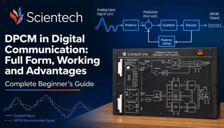
A DPCM transmitter typically includes a sampler, subtractor, quantizer, predictor, and encoder, along with a feedback path from the reconstructed sample to the predictor.

governing equations:

e(nTs) = x(nTs) − x̂(nTs)

v(nTs) = Q[e(nTs)] = e(nTs) + q(nTs), where q(nTs) is quantization error

u(nTs) = x̂(nTs) + v(nTs)

u(nTs) is a reconstructed sample fed back into the predictor. Only v(nTs), the quantized prediction error, is encoded and sent over the channel. Substituting shows u(nTs) = x(nTs) + q(nTs): the reconstructed sample equals the original sample plus quantization error, which is the expected result of quantization in a lossy system.

DPCM Receiver: Reconstruction

receiver decodes bitstream to recover v(nTs) and runs a predictor identical in structure to transmitter’s. It computes:

u(nTs) = x̂(nTs) + v(nTs)

u(nTs) becomes both output sample (after D/A conversion and low pass filtering) and input to receiver’s own predictor for next cycle. Since the transmitter and receiver run the same prediction logic on the same reconstructed data, the two stay aligned without ever exchanging raw sample values.

This symmetry is also DPCM’s main liability. Because each prediction depends on previous reconstructed samples, a quantization error in one sample changes the reconstructed value used for later predictions. This can affect the prediction errors and reconstructed samples that follow. In practice, this can cause a burst of distortion that may continue for several subsequent samples. How quickly the effect dies out depends on the predictor and system design.

Worked Example: Bit Rate Reduction

Problem: A signal is sampled at 8,000 samples/second. Standard PCM requires 8 bits per sample. Using DPCM, prediction error requires only 4 bits per sample. Find bit rate for both schemes and percentage reduction.

PCM bit rate = 8,000 × 8 = 64,000 bps = 64 kbps

DPCM bit rate = 8,000 × 4 = 32,000 bps = 32 kbps

Percentage reduction = (64,000 − 32,000) / 64,000 × 100 = 50%

DPCM halves the bit rate in this example because the assumed prediction error can be represented using 4 bits per sample, compared with the 8 bits per sample used by PCM.

A second variant to try yourself: if same signal is sampled at 8,000 samples/second but prediction error now needs 5 bits per sample (a weaker predictor, larger residual), DPCM bit rate becomes 8,000 × 5 = 40,000 bps, a 37.5% reduction over PCM instead of 50%. bit savings scale directly with how good a predictor is, not just with the fact that DPCM is being used at all.

PCM vs DPCM vs DM vs ADPCM

DM is a special case of DPCM with a 1 bit quantizer: output only signals whether signal moved up or down by a fixed step Δ. Its two characteristic failure modes are slope overload, when input changes faster than Δ can track, and granular noise, when input is nearly flat but fixed step causes it to oscillate around true value.  ADPCM can reduce these problems by adapting the step size to recent signal behaviour: larger steps during fast transitions and smaller steps when the signal is relatively steady.

Where DPCM Is Used :

DPCM and its variants are used where consecutive samples are strongly correlated and bandwidth is limited. Two well documented cases:

Speech coding. ITU T’s G.726 standard specifies ADPCM for digital telephony at 16, 24, 32, and 40 kbit/s, directly building on DPCM principle covered here.

Lossless and near lossless image compression. Predictive coding is also used in image compression. JPEG’s lossless mode encodes prediction errors, while JPEG-LS uses a more advanced predictive coding approach designed for lossless and near-lossless compression. (JPEG). Modern video codecs (H.264, HEVC) use much more sophisticated motion compensated prediction, but the underlying idea of predict then encodes the residual traces back to DPCM.

Be careful not to overstate this: modern speech and video codecs are not “DPCM systems.” They may combine predictive coding with other techniques such as transform coding and entropy coding. Video codecs can also use motion estimation and motion compensation. DPCM is a foundational concept, not a full picture of how a modern codec works.

Conclusion

DPCM transmitter reduces bit rate by predicting each sample from its reconstructed history and transmitting only residual. A predictor feedback structure that makes this possible is also the reason errors can propagate, which is the main design trade off engineers manage when choosing predictor order and quantizer step size. Delta Modulation and ADPCM are related to the same predictive-coding idea. DM uses a 1-bit decision to indicate whether the signal should move up or down, while ADPCM adds adaptation to the prediction and/or quantization process.

Frequently Asked Questions About DPCM